It has been a month since my last post where I introduced you to the work that we’ve been doing with embeddings in Orcasound datasets. This time I want to present more deeply the concepts and the experiments that we did, and also share with you some updates on my project.

Two key concepts have been bouncing around in my head during the development of this project: representation and similarity. How are those concepts formally defined? If we look for the dictionary definition of “similar” it states “like somebody/something but not exactly the same,” so being similar is essentially a relationship between entities or objects, a relationship of closeness which also implies that there are small perturbations that make the entities “not exactly the same.”

How do we measure that a sound is similar/close to another?

Here’s when the second concept enters into play… representation. A representation is an abstraction that we make about an object that encapsulates meaning, is a “summary” of the object. Different representations can exist for the same object, each with different purposes. We would say that we need a representation to be able to measure how similar a sound is to another.

How do we construct representations, and specifically sound representations?

There’s a way of building representations using characteristics or features of the objects. Let’s take the example of a trumpet note. We could measure the duration of the note, the fundamental frequency (that defines a musical note, e.g. C#), the harmonics of the sound, or the loudness. However, each of these characteristics serves a different purpose. For example, the duration of the sound is not useful in determining if the note is a C or D, but the duration of the sound in another context could allow us to differentiate between a gong sound that has a long decay and a snare drum that has a smaller decay (unless is affected by and 80’s reverb ;).

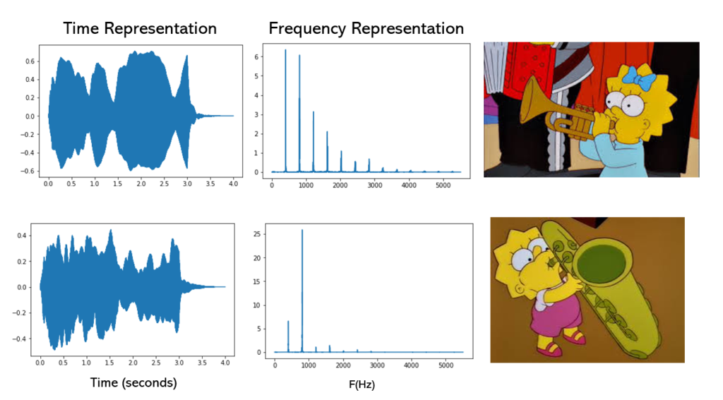
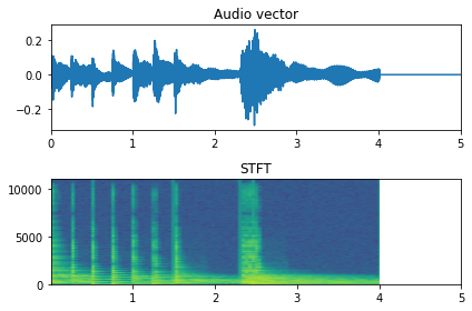
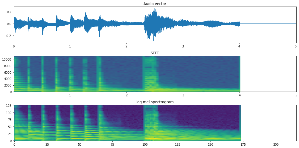
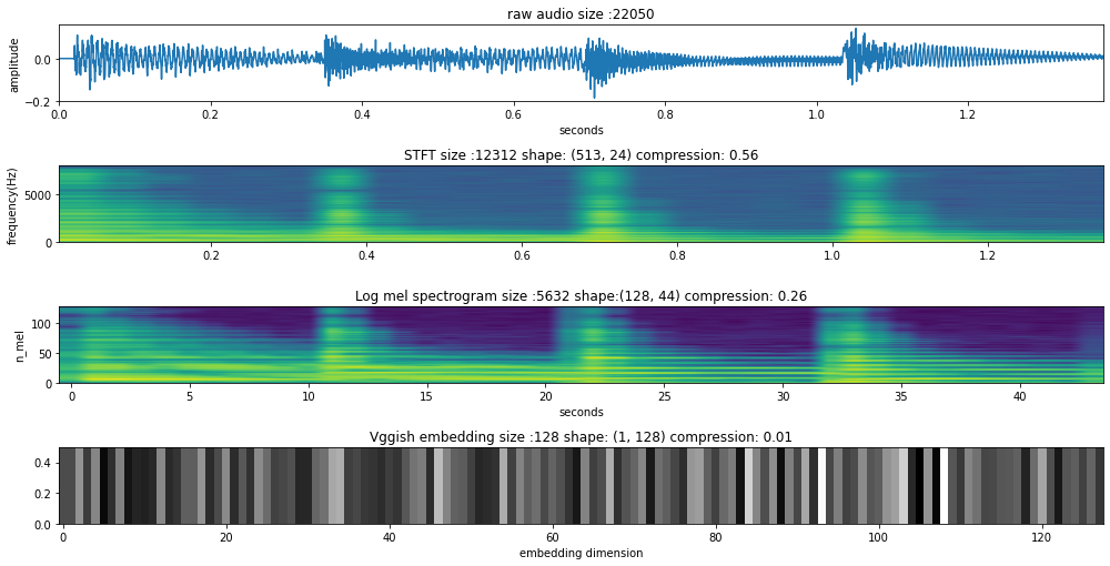
In computers, we represent sound as a 1-d vector of discrete values, which are the digitized version of the sound’s pressure variations (in air or seawater, or any medium) that are sensed by a microphone or hydrophone. This time series of pressure amplitude measurements is the time waveform representation, also called the raw audio. Another representation of sound is the DFT (discrete Fourier transform) that allows us to see the frequency content of the signal. However, as sounds have duration, those DFT can be stacked to form a matrix that captures the evolution of the frequency in time. This representation is called STFT (Short-time Fourier transform).

Nowadays, a lot of audio AI models rely on another time-frequency representation that applies a psychoacoustic derived filterbank to the STFT and is called the log-mel spectrogram. It is important to say that these representations have parameters associated with them — like the window size, the hop size, number of mels — that change the size of the representation.

There is a fourth representation which is the one that we’ve been working on: the embedding. In the last post, I defined an embedding when it is derived from a neural network, however, a better definition would be:

An embedding is a representation of a topological object, manifold, graph, field, etc. in a certain space in such a way that its connectivity or algebraic properties are preserved.

Insall, Matt; Rowland, Todd; and Weisstein, Eric W. “Embedding.” From MathWorld–A Wolfram Web Resource

Therefore, for a second of audio, we have four representations with different sizes being the raw audio the bigger representation and the embedding the smaller one. We can think of this representation as a form of information compression because we are representing the same second of audio with 1% of the size of the raw audio.

What properties is the embedding preserving? And is any sound semantic tied to those properties?

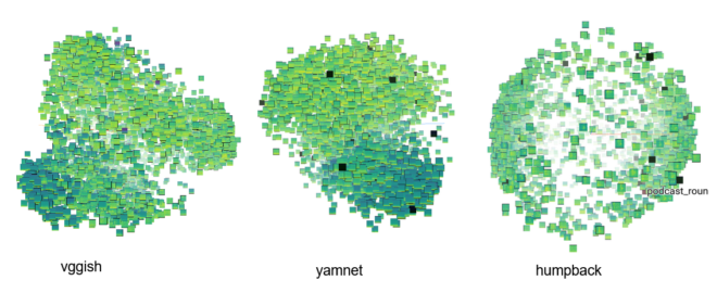
Those questions take us to do a bunch of experiments using a subset of the Orcasound datasets that has the positive labels of orca calls. We use 3 embeddings models that output vectors of 128,1024 or 2048 per second respectively vggish, yamnet and humpack_whale.

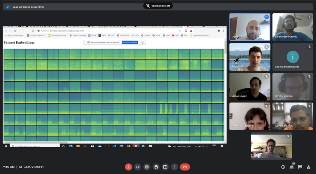
We extract those embeddings on each audio clip of the dataset so that an audio clip is represented by an N-dimensinoal vector, where N depends on the model chosen. As you can see, it is difficult to figure out the meaning of the embedding itself; we aren’t used to understanding spaces that have more than 3 dimensions. Therefore, we use some dimensionality reduction techniques that are available in the embedding projector tool to represent the 128, 1024 or 2048 vectors into a 3-dimensional space. As an additional aid, instead of plotting points, we plot the spectrogram representation of the audio to easily inspect how the patterns and the structure of the embedding space correlate with the audio content.

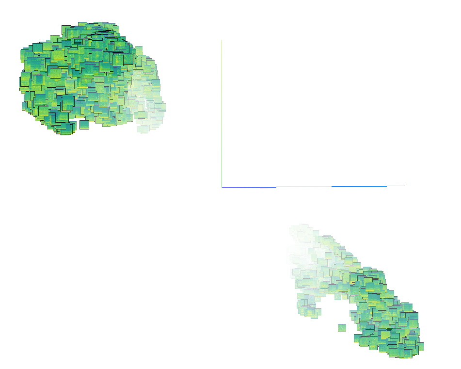
We obtained the plot above that is showing 4900 audio clips using a dimensionality reduction technique called PCA (principal component analysis). This technique aims to maximize the variance using linear projections of the original dimensions. For the vggish, and yamnet model we obtained explained variances close to 40% with the first 3 components, telling us that we’re missing details of the structure of the original space, despite the fact that we can see that similar spectrograms are closer together. For the humpback model, the explained variance is close to 80% and we identify 2 big clusters, so the original space is trying to separate all of the examples into 2 groups. This is really interesting as the humpback whale embeddings came from a binary classification model.

We chose to focus on a subset of the dataset that has recordings from only one location, as the global structure of the yamnet and vggish models is mainly explained by the location of the recording. There is also another dimensionality reduction technique called t-SNE

Roughly, what t-SNE tries to optimize for is preserving the topology of the data. For every point, it constructs a notion of which other points are its ‘neighbors,’ trying to make all points have the same number of neighbors. Then it tries to embed them so that those points all have the same number of neighbors. (See https://colah.github.io/posts/2014-10-Visualizing-MNIST/ )

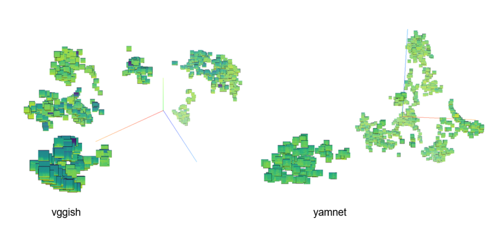
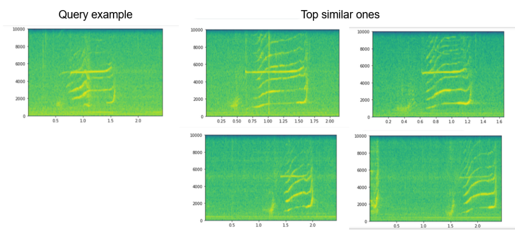
Now we can see some clusters with very similar spectrograms that are possibly the same type of orca calls. Thus, the embedding representation is allowing us to group similar sounds. Finally, those two concepts acquire a sense in our experiment. We also perform some queries on the whole dataset using the embedding to retrieve the 5 nearest sounds to a given sample and the results using subjective listening tests were satisfactory.

If you are interested in doing this kind of exploration on audio databases, you can visit the repo where I have been working this summer. It has instructions on how to publish your own experiments on the embedding projector and some helper functions to extract the embeddings.

I also want to mention that we had the opportunity to present our ongoing work in the HALLO project call. It was very enjoyable to meet other scientists passionate about bioacoustic analysis and conservation, and also a great networking opportunity.

I want to thank my mentors Valentina, Jesse, Scott, Kunal and Val for taking the time to discuss and explore these datasets in a detailed way and for the valuable feedback and suggestions to improve the project that I have received from them. Last but not least go and listen to the sea sounds live.