I am Kunal Mehta currently in my final year of Computer Engineering in Mumbai, India. I am passionate about the concepts of Machine Learning and Deep Learning and especially the Mathematics behind it. I was selected as a Google Summer of Code 2020 student for Orcasound and am working with another student, Diego, on developing an active learning tool.

The Southern Resident Killer Whales (SRKW) that lives along the coast of the Pacific Northwest are critically endangered and it is becoming extremely important to save them. Therefore, it is very important to detect these SRKWs and one way to detect them is acoustically — by identifying the sounds or calls made by the orcas — and automatically, using a machine learning model known as a Convolutional Neural Network (CNN).

Orcasound has placed their hydrophones at various locations which would capture the calls and other sounds from the ocean. Some recordings of SRKW calls from these locations have been labeled through the open-source Pod.Cast tool (developed through Microsoft hackathons) which generates a .tsv file that contains multiple parameters like start_time, duration, location, etc of the calls. We are going to generate spectrograms from these data to train a CNN model and then tune the hyperparameters such that overall good accuracy is achieved.

With a basic model trained on Orcasound data, the next step in my summer GSoC project is the Active Learning Phase which we are going to perform this month. Here is a diagram of the active learning pipeline in which a human user will iteratively validate a model output to help it learn faster than through other methods.

• 

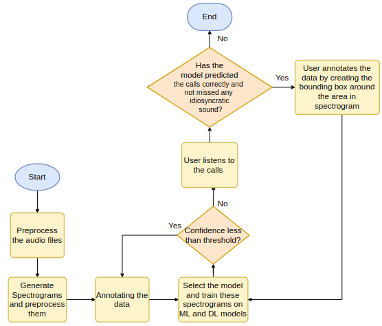
The above pipeline consists of multiple stages:

1. Preprocessing Stage
   In this phase, we would preprocess the audio data and spectrograms such that it is convenient to be fed to the model. There are three preprocessing cases that we experimented with and used which is explained in detail below.
2. Model creation and training stage
   In this phase, we created a model that would be able to identify the Orca calls with good accuracy. Different models have been tried and tested and the result of each model’s accuracy and loss is shown below.
3. Building an Active Learning tool with the help of ModAL library on a model created in stage 2
4. Detecting the Orcas and training the model again on the labels generated by the Active Learning tool.

I’ve made a first pass through stages one and two during June. Stages three and four are scheduled for this month.

This blog describes in more detail the first two stages:
1. Preprocessing
2. Creating a model

Stage 1: Preprocessing

The Orcasound organization had taken tremendous efforts and generated the training data and testing data for us which consisted of the audio files containing the calls and a .tsv file containing various parameters like the start-time, duration, location, and many other parameters of the calls. I utilized those data to perform preprocessing and generate spectrograms.

In the .tsv file, the thing that I was most interested in was the start time and the duration of the call. With them, I was planning to extract calls in short clips that contained only true orca calls. The non-orca calls were also generated from the same audio file, thanks to the Ketos library which has a background sound generator that would create a .csv file containing the areas that are not within the start time and duration of the calls. Using any area that is not within the start time and duration of the call to define the background sounds, I extracted those periods as audio files not containing orca calls.

Thus, now I have both positive call data containing only the audio clip with the call and negative call data which had only contain background noise. All these audio files are later converted to spectrograms. There are three different cases in which I tried to determine the best spectrograms in the preprocessing stage to generate a model that achieves maximum accuracy.

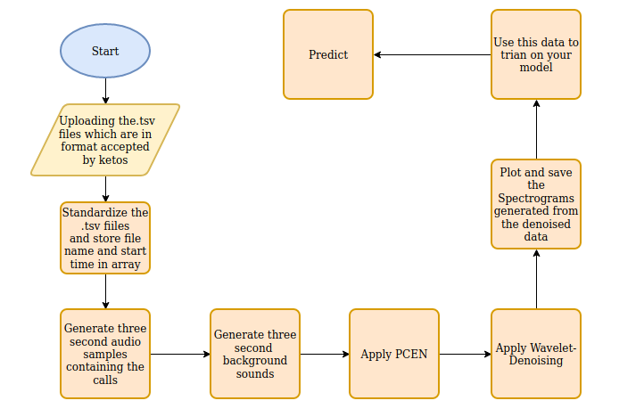
In case one, the spectrograms are plotted from the raw audio (both call and no-calls audio files). The same is true for cases two and three, but in case two I am also using  per-channel energy normalization (PCEN) as a preprocessing stage, and for case three I am applying both PCEN and Wavelet Denoising on the spectrograms.

This is how we generated different spectrograms by three processing methods. Now these spectrogram images can used to train models and find the best one (and therefore decide which preprocessing is optimal for detecting orca signals).

Please note that the above diagram is only for case three and all the cases and steps are explained in complete detail in the active learning backend github repository.

Stage 2: Model Creation

Different models have been tried on different cases as seen in the first flowchart. The number of training samples was 1394 images and there were 201 test data samples I used to assess model performance. Below I have explained models that have been tried in each of the preprocessing cases.

Case 1: No preprocessing

Model 1: VGG16 model was fine-tuned to be trained on spectrograms of calls and no calls. The model was overfitting, both the ones that was pretrained on imagenet data and the one trained from scratch (i.e all the layers of VGG16 model were trained). This might be because of the large number of layers in the complex model was not able to generalize well on the small amount of dataset.

Model 2: Simple CNN with four convolution layers was used which performed comparatively better than the VGG16 model, with accuracy around 74% on the test data.

Case 2: Preprocessing using PCEN

Model 1: VGG16 model was fine-tuned, but, not surprisingly the results turned out to be similar to the ones generated from case 1. The model was overfitting and the predictions on the test dataset were not accurate.

Case 3: Preprocessing using PCEN and Wavelet Denoising

Model 1: VGG16 model was as usual overfitting but if the data is more it might be the most useful model.

Model 2: Resnet-512 model performed similar to VGG16 with slightly higher accuracy on the test data.

Model 3: InceptionResnet-V2 model performed quite better than both these models but still it was not the best but an increase in training data would make this model one of the best models for training.

Model 4: Simple four-layer Convolution Neural Network would win the battle since due to small data the model is generalized well and has some pretty good accuracy without overfitting.

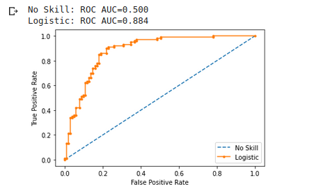
Here is the confusion matrix of the Simple Convolution Neural Network that I used:

Found 201 images belonging to 2 classes.
              precision    recall  f1-score   support

       calls       0.85      0.80      0.83       101
     nocalls       0.81      0.86      0.83       100

    accuracy                           0.83       201
   macro avg       0.83      0.83      0.83       201
weighted avg       0.83      0.83      0.83       201

[[81 20]
 [14 86]]
acc: 0.8308
sensitivity: 0.8020
specificity: 0.8600

But, creating and tuning this Convolution Neural Network was the most difficult task, as when I initially used a four-layer CNN without dropout it reached an accuracy of 1.0000 within 22 epochs and was overfitting as the predictions on the test data were less than 54%.

Then I tried to add some L2 regularizers, as I thought it might reduce the overfitting, but alas it just helped a little and my predictions on test data had accuracy around 62%. But the accuracy of the training data was still reaching to one.

Now it was time to add the dropout along with regularizers and this time the model worked quite well! The above-generated accuracy was from this particular model.

Here is the summary of different models with different parameters.

model	test	test description	total params	trainable params	non-trainable params	epochs	steps per epoch	training accuracy	loss
VGG-16	case-1	no preprocessing applied	134,268,738	8,194	134,260,544	238	8	0.8881	0.2632
Basic-CNN	case-1	no preprocessing applied	6,079,937	6,079,937	0	5	1570	0.9746	0.075
VGG-16	case-2	PCEN applied	134,268,738	8,194	134,260,544	62		1	2.95E-05
VGG-16	case-3	PCEN and wavelet denoising	134,268,738	8,194	134,260,544	238		0.9995	0.0222
Basic-CNN-1	case-3	PCEN and wavelet denoising	12,371,393	12,371,393	0	3	1570	0.5007	-134067011115
ResNet-512	case-3	PCEN and wavelet denoising	58,532,354	58,532,354	58,532,354	41	50	0.8438	2.0311
Basic-CNN-2	case-3	PCEN and wavelet denoising	2,819,649	2,819,649	0	550	8	0.9741	0.0674

• 

Thus, a good model that can be used for active learning has been built. How we use theses models to create an active learning pipeline will be seen in my next blog post!

Thanks for your time and efforts for reading this blog. I hope you found it helpful!