
Analysis of Fourier Transforms techniques for underwater denoising
Effective denoising strategies for underwater background noise, according to the paper by Akshada N. et al [1], include:
- Least Mean Square
As the Least Mean Square algorithm require target values to adapt and we do not have reference denoised audios yet, this algorithm has not applicable now. - Fourier Transform filters and Short Time Fourier Transforms filters
- Discrete Wavelet Transform
- Empirical Mode Decomposition
Here, we provide the findings of comparing several Fourier Transform methods on two sets of orca calls. The first set contains a single 25-second audio clip, while the second set has five audio samples with varying lengths, orca calls, and noise levels. These are the links for the single audio clips and the 5 audio clips.
Fourier Transforms
We considered the most Fourier Transform filters for signal smoothing and denoising [2]:
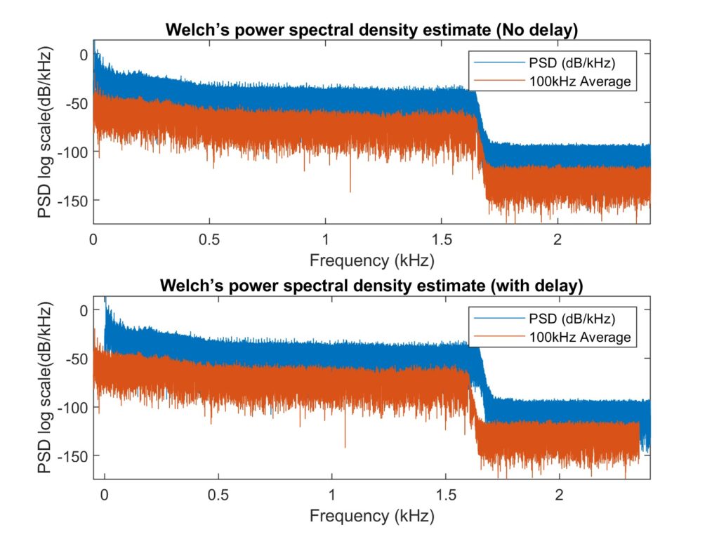
- Moving average filter (with steps of 100 Hz, accounting for a delay of half step)[2]
- Moving weighted average filters [2] (binomial and exponential weighting/gaussian e)
- Savitzky-Golay filters (fitted using cubic, quartic and quintic polymials [3])
- Median Average (fitted with polynomial of degrees 2, 10, 12 [4])
- Hampel Filter [5]
Methods
The single clip from the first set is an encounter between a humpback and Bigg’s killer whales in the Salish sea [6].
The 5 clips from the second set, on the other hand, were randomly selected from the acoustic sandbox training dataset from among those that had annotated orca sounds [7].
Both sample sets have been evaluated qualitatively because there aren’t any reference denoised clean audios to compare them to. For the second set, we computed Signal-to-Noise-Ratio, Mean Squared Error and Root Mean Squared Error between the denoised and original audio clip.
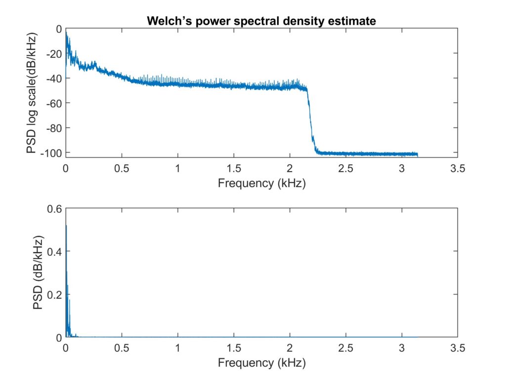
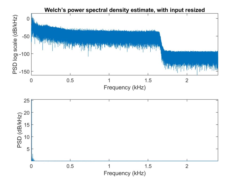
For the first set calculated the original and denoised signals’ Welch’s power spectral densities for each method. All signal lengths were normalised to be a power of two. In contrast to a large prime factor, scaling the signal size as a power of 2 makes it computationally quicker [8].
We used the binomial moving average, the moving average filter, and the median average filter to compare performances for the set of 5 clips. The median filter and the Hampel filter were the two that performed the best in the single clip experiment, so we decided to use one of them for this set. However, for the collection of 5 clips, the binomial moving average and the moving average did the best audibly, therefore we selected these 2.
Results and discussion
Single clip set
I determined from the spectral density graphs that it appears to be a mirrored step function, therefore frequency domain thresholding would not be effective. These are the links for the filtered audio clips and the plots.
- Moving average filter
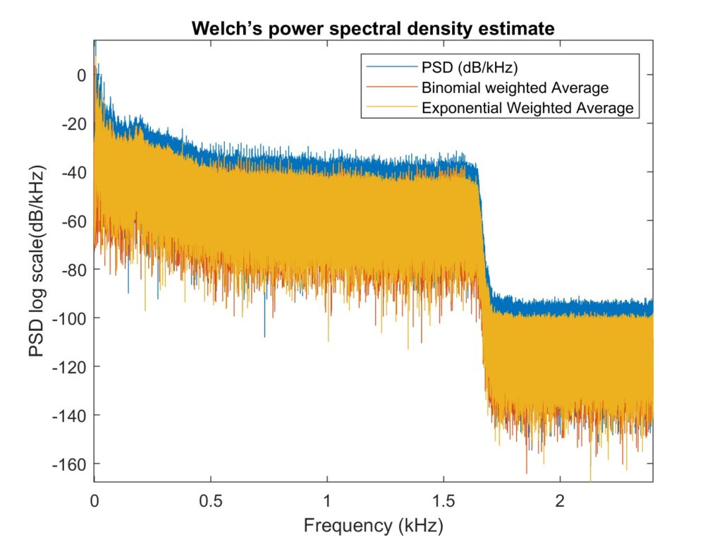
Here, I made a comparison of with the delay of the half step and without it. - Moving weighted average filters
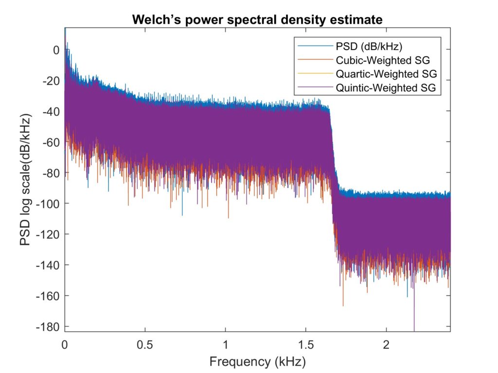
The binomial weighting fits the original signal tighter compared to the exponential weighting - Savitzky-Golay filters
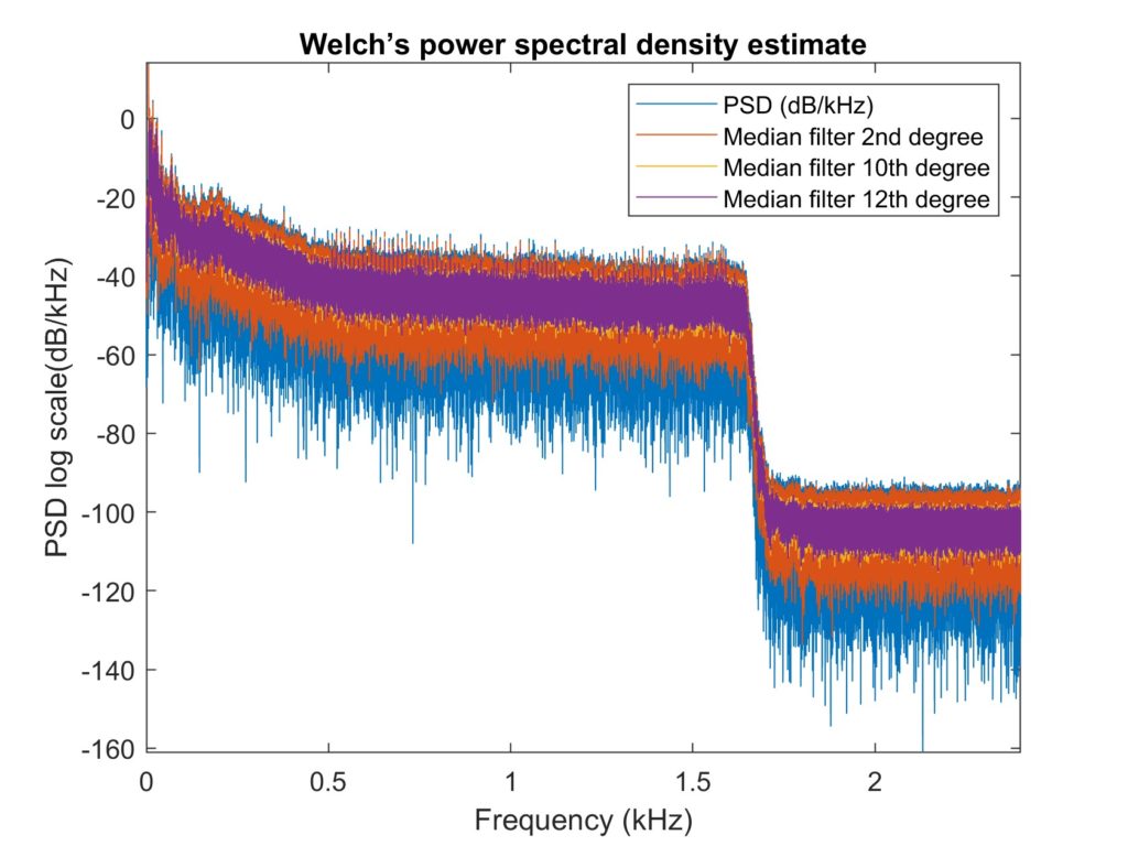
In comparison to the 3rd and 4th degree polynomials, the 5th degree polynomial fits better. - Median filters
Different polynomial degrees produced results that were similar, therefore I believe adopting the lowest degree of 2 is sufficient. - Hampel filter
The Hampel filter replaces outliers with values that are equivalent to a few standard deviations from the median as opposed to the median filter. Consequently, it performed similarly to the median filter.
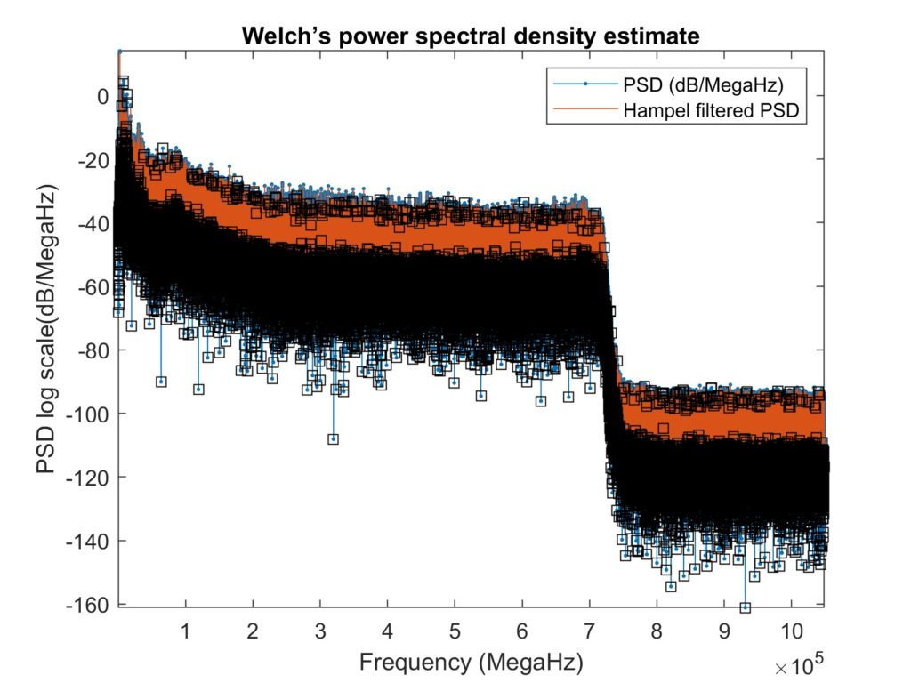
Due to the regular shape of the original signal power, the median filter and the Hampel filter performed the best for the first set.
5 clips set
| Mean across clips | SNR | MSE | RMSE |
|---|---|---|---|
| Binomial moving average filters | -0.8267 | 216.2142 | 13.8225 |
| Moving average filter | -0.9858 | 193.1446 | 12.9034 |
| Median filter | -0.3356 | 556.8749 | 21.8629 |
The metrics for this set were not relevant since the denoised audios had higher metric values the more boat noises they contained. The orca vocalisations were really mistaken for noise. The full metric results are in this Google doc [9] and this is the link for the denoised audio clips.
Conclusion
Both experiments have led me to the conclusion that the technique that worked best for a single clip was not the best for a set of five clips. We cannot select a single Fourier transform technique as the best due to the variation in noise levels among samples. In the next post we will analyse the performance of Discrete Wavelet Transforms for denoising.
Bibliography
[1] Kawade, A.N. and Shastri, R.K., 2016. Denoising techniques for underwater ambient noise. Int. J. Sci. Technol. Eng, 2(7), pp.150-154.
[2] 2022. [online] Available at: https://uk.mathworks.com/help/signal/ug/signal-smoothing.html [Accessed 4 August 2022].
[3] 2022. [online] Available at: [Accessed 4 August 2022].
[4] 2022. [online] Available at: https://uk.mathworks.com/help/signal/ref/medfilt1.html#buu8gnt-3 [Accessed 4 August 2022].
[5] 2022. [online] Available at: [Accessed 4 August 2022].
[6] 2022. [online] Available at: https://www.orcasound.net/2018/12/02/humpback-and-biggs-killer-whales-serenading-in-the-darkness/ [Accessed 4 August 2022].
[7] 2022. [online] Available at: [Accessed 4 August 2022].
[8] 2022. [online] Available at: https://uk.mathworks.com/help/matlab/math/basic-spectral-analysis.html [Accessed 4 August 2022].
[9] 2022. [online] Available at: https://docs.google.com/document/d/1fIpVqpbVsaaXW0neziQKhy4vG3QMsNyEjGIX1KY7W0A/edit?usp=sharing [Accessed 4 August 2022].